set samples 2001
set terminal postscript enhanced landscape color lw 2 "Times-Roman" 20
set output "butterworth.ps"

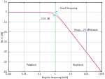
# Butterworth amplitude response and decibel calculation.  n is the order, which is just 1 in this image.
G(w,n) = 1 / (sqrt(1 + w**(2*n)))
dB(x) = 20 * log10(abs(x))

# Gridlines
set grid

# Set x axis to logarithmic scale
set logscale x 10

# Set range of x and y axes
set xrange [0.001:1000]
set yrange [-60:10]

# Create x-axis tic marks once per decade (every multiple of 10)
set xtics 10

# Use 10 x-axis minor divisions per major division
set mxtics 10

# Axis labels
set xlabel "Angular frequency (rad/s)"
set ylabel "Gain (dB)"

# No need for a key
set nokey #0.1,-25

# Frequency response's line plotting style
set style line 1 lt 1 lw 2

# Draw a separator between passband and stopband and label them
set style line 2 lt 2 lw 1
set style arrow 2 nohead ls 2
set arrow 3 from 1,-60 to 1,10 as 2

# Label coordinates are relative to the graph window, not to the function, centered at the 1/4 and 3/4 width points
set label 1 "Passband" at graph 0.25, graph 0.1 c
set label 2 "Stopband" at graph 0.75, graph 0.1 c

# Asymptote lines and slope lines are the same "arrow" style
set style line 3 lt 3 lw 1
set style arrow 3 nohead ls 3

# Draw asymptote lines
set arrow 1 from 1,0 to 1000,-60 as 3
set arrow 2 from .001,0 to 1,0 as 3

# -3 dB arrow style and arrow
set style line 4 lt 4 lw 1
set style arrow 4 head filled size screen 0.02,15,45 ls 4
set arrow 4 from 2,3 to 1,0 as 4

# "Cutoff frequency" label uses same coordinates as the function
set label 3 "Cutoff frequency" at 2,4 l

# "-3 dB" label
set arrow 5 from 0.5,-6 to 1,-3 as 4
set label 4 "-3.01 dB" at 0.5,-7 r

# Draw slope lines and label
set arrow 6 from 100,-20 to 12,-20 as 3
set arrow 7 from 100,-20 to 100,-39 as 3
set label 5 "Slope: -20 dB/decade" at 100,-18 c

# Plot the filter response
plot \
     dB(G(x,1)) ls 1  title "1st-order response"


